21 February 2018
In this exercise, we are going to explore the model put forth by Clark and Cummins (2015) explaining intergenerational correlations in wealth. A typical intergenerational wealth elasticity estimate is based on the assumption that son’s wealth is related to father’s wealth through the following linear equation:
\[\begin{equation} w_{i,t+1} = \beta w_{i,t} + \nu_{i,t} \end{equation}\]However, Clark and Cummins are going to argue that it is really an underlying social status, \(x_{i,t}\), and a random component, \(u_{i,t}\), that determine wealth and that it is this underlying social status that is linked across generations. In particular, they assume that wealth is given by:
\[\begin{equation} w_{i,t} = x_{i,t} + u_{i,t} \end{equation}\]and that underlying social status is transmitted across generations according to:
\[\begin{equation} x_{i,t+1} = b x_{i,t} + e_{i,t} \end{equation}\]where \(e_{i,t}\) is a random component with mean zero. We are going to simulate wealth across several generations using these equations to see how the value of \(b\) and the distributions of \(u_{i,t}\) and \(e_{i,t}\) influence the evolution of wealth over several generations (and our traditional estimate of \(\beta\) in the first equation above).
First, let’s construct a sample of our first generation and match the distribution of their wealth to the actual British wealth data used by Clark and Cummins:
. clear

. set obs 5000
number of observations (_N) was 0, now 5,000

. gen id = _n

. gen log_wealth_gen1 = rnormal(2.24,1.72)
The set obs command generates an empty 5,000 observation dataset. The gen id command simply creates a unique id number for each observation equal to its observation number. Finally, we generate log wealth as a random variable using Stata’s rnormal function. The mean and standard deviation for log wealth are taken from Table 1 of Clark and Cummins (2015).
We have matched the observed log wealth distribution, but what we really care about is the distribution of this underlying social status \(x_{i,t}\). Let’s assume that both \(x_{i,t}\) and \(u_{i,t}\) are normally distributed and independent of one another. In that case, \(w_{i,t}\), as the sum of two normally distributed random variables, will also have a normal distribution given by:
\[\begin{equation} w \sim N(\mu_{x}+\mu_{u}, \sigma_{x}^{2} + \sigma_{u}^{2}) \end{equation}\]We are assuming that \(\mu_{u}\) is zero, so the mean of \(x_{i,t}\) should be the same as the mean of log wealth. As for the \(\sigma_{x}\) and \(\sigma_{u}\), picking a value for one will let us calculate the value for the other given the observed \(\sigma_{w}\). Let’s calculate and store these values using a couple local macros and then generate our \(x\) values for the first generation:
. local sigma_x = 1

. local sigma_u = (1.72^2 - `sigma_x'^2)^.5

. gen x_gen1 = log_wealth_gen1 - rnormal(0,`sigma_u')
Now that we have our \(x_{i,t}\) variable, we can start simulating subsequent generations. Let’s create a total of five generations. To do so, we need to pick a value for \(b\), the parameter linking social status across generations and a value for the standard deviation of \(e_{i,t}\), the random component of social status. We’ll start with the following fairly arbitrary choices:
. local b = 0.5

. local sigma_e = 1
Now we have everything needed to start simulating the generations:
. gen x_gen2 = `b'*x_gen1 + rnormal(0,`sigma_e')

. gen log_wealth_gen2 = x_gen2 + rnormal(0,`sigma_u')

. gen x_gen3 = `b'*x_gen2 + rnormal(0,`sigma_e')

. gen log_wealth_gen3 = x_gen3 + rnormal(0,`sigma_u')

. gen x_gen4 = `b'*x_gen3 + rnormal(0,`sigma_e')

. gen log_wealth_gen4 = x_gen4 + rnormal(0,`sigma_u')

. gen x_gen5 = `b'*x_gen4 + rnormal(0,`sigma_e')

. gen log_wealth_gen5 = x_gen5 + rnormal(0,`sigma_u')
Let’s see what we get when we regress fifth generation wealth on fourth generation wealth:
. reg log_wealth_gen5 log_wealth_gen4

      Source │       SS           df       MS      Number of obs   =     5,000
─────────────┼──────────────────────────────────   F(1, 4998)      =    201.94
       Model │  655.934388         1  655.934388   Prob > F        =    0.0000
    Residual │   16234.077     4,998  3.24811465   R-squared       =    0.0388
─────────────┼──────────────────────────────────   Adj R-squared   =    0.0386
       Total │  16890.0114     4,999  3.37867802   Root MSE        =    1.8023

────────────────┬────────────────────────────────────────────────────────────────
log_wealth_gen5 │      Coef.   Std. Err.      t    P>|t|     [95% Conf. Interval]
────────────────┼────────────────────────────────────────────────────────────────
log_wealth_gen4 │   .2000541   .0140777    14.21   0.000     .1724556    .2276527
          _cons │   .0744448   .0257713     2.89   0.004     .0239216    .1249679
────────────────┴────────────────────────────────────────────────────────────────
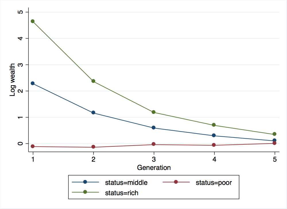
Notice that the coefficient is smaller than our chosen value of \(b\). In other words, the observed correlation in wealth across two generations is much smaller than the underlying correlation in social status across generations. To look at how rich and poor families are reverting to the mean, let’s define three groups: rich, middle and poor corresponding to the top, middle and bottom wealth quintiles of the first generation:
. sort log_wealth_gen1

. gen status = ""
(5,000 missing values generated)

. replace status = "rich" in 4001/5000
variable status was str1 now str4
(1,000 real changes made)

. replace status = "middle" in 2001/3000
variable status was str4 now str6
(1,000 real changes made)

. replace status = "poor" in 1/1000
(1,000 real changes made)
Now we can graph their evolution over time, although it will be easier to do so if we first reshape the data, putting it in long format. After reshaping the data, we can use the binscatter package to make a graph:
. reshape long log_wealth_gen x_gen, i(id) j(generation)
(note: j = 1 2 3 4 5)

Data                               wide   ->   long
─────────────────────────────────────────────────────────────────────────────
Number of obs.                     5000   ->   25000
Number of variables                  12   ->       5
j variable (5 values)                     ->   generation
xij variables:
log_wealth_gen1 log_wealth_gen2 ... log_wealth_gen5->log_wealth_gen
               x_gen1 x_gen2 ... x_gen5   ->   x_gen
─────────────────────────────────────────────────────────────────────────────

. binscatter log_wealth generation, by(status) linetype(connect) xtitle("Generation") ytitle("Log wealth")
(10000 missing values generated)

. graph export wealth_across_five_generations.png, width(500) replace
(file wealth_across_five_generations.png written in PNG format)
So the rich are still rich after five generations, but not by much. Now we have everything in place to explore how the various parameters (\(b\), \(\sigma_{e}\), \(\sigma_{u}\)) influence wealth mobility across generations and our estimates of \(\beta\). An easy way to do this is to write a short do file that will generate all of our \(x\) and \(w\) values after we set the parameters. I’ve created one such do file, simulate-wealth.do, available here. This do file contains all of the commands we used above except for setting the local macros for \(b\), \(\sigma_{x}\) and \(\sigma_{e}\) (recall that \(\sigma_{u}\) was determined by our choices of \(\sigma_{x}\) and \(\sigma_{w}\)) and for the final graphing step. Let’s give it a try, using the same values for \(\sigma_{e}\) and \(\sigma_{x}\) but a new higher value for \(b\):
. local sigma_x = 1

. local b = 0.75

. local sigma_e = 1

. quietly do simulate-wealth.do `sigma_x' `b' `sigma_e'
Notice that I added quietly when issuing the do command. This suppresses output while the do file runs, keeping our results screen from getting too cluttered. Also notice that I needed to include the local macro names that the do file will use. If you do not do this, any commands within the do file cannot see the local macros generated outside of the do file. When referencing these local macros within the do file, you refer to them by the order in which you listed them (so `sigma_x’ is referenced as `1’, `b’ is referenced as `2’ and `sigma_e’ is referenced as `3’).
Now that we have simulated new wealth values with a higher value for \(b\), let’s see how our estimate of \(\beta\) and our graph of wealth across generations have changed:
. reg log_wealth_gen5 log_wealth_gen4

      Source │       SS           df       MS      Number of obs   =     5,000
─────────────┼──────────────────────────────────   F(1, 4998)      =   1193.53
       Model │  4360.48947         1  4360.48947   Prob > F        =    0.0000
    Residual │  18259.9496     4,998  3.65345131   R-squared       =    0.1928
─────────────┼──────────────────────────────────   Adj R-squared   =    0.1926
       Total │  22620.4391     4,999  4.52499282   Root MSE        =    1.9114

────────────────┬────────────────────────────────────────────────────────────────
log_wealth_gen5 │      Coef.   Std. Err.      t    P>|t|     [95% Conf. Interval]
────────────────┼────────────────────────────────────────────────────────────────
log_wealth_gen4 │   .4334626   .0125469    34.55   0.000     .4088653      .45806
          _cons │   .3210471   .0296924    10.81   0.000      .262837    .3792571
────────────────┴────────────────────────────────────────────────────────────────

. reshape long log_wealth_gen x_gen, i(id) j(generation)
(note: j = 1 2 3 4 5)

Data                               wide   ->   long
─────────────────────────────────────────────────────────────────────────────
Number of obs.                     5000   ->   25000
Number of variables                  12   ->       5
j variable (5 values)                     ->   generation
xij variables:
log_wealth_gen1 log_wealth_gen2 ... log_wealth_gen5->log_wealth_gen
               x_gen1 x_gen2 ... x_gen5   ->   x_gen
─────────────────────────────────────────────────────────────────────────────

. binscatter log_wealth generation, by(status) linetype(connect) xtitle("Generation") ytitle("Log wealth")
(9990 missing values generated)

. graph export wealth_across_five_generations_b.png, width(500) replace
(file wealth_across_five_generations_b.png written in PNG format)
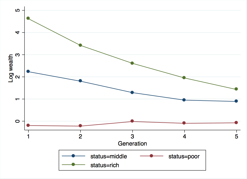
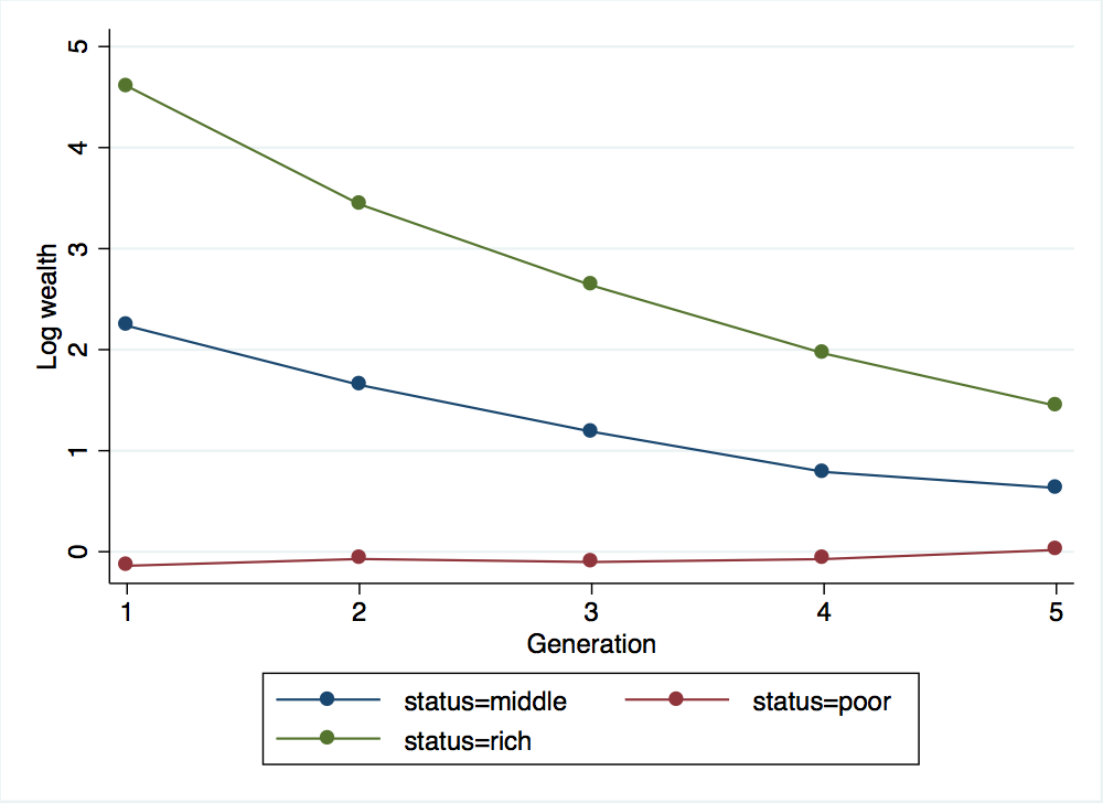
As expected, a larger value of \(b\) led to a larger estimated value for \(\beta\) in the regression. From the graph, it is clear that the higher value for \(b\) is leading to much slower reversion to the mean. Now, keeping \(b\) at 0.75, let’s see what happens if we try a much smaller variance for \(x\) and a much larger variance for \(x\):
. local sigma_x = .25

. local b = 0.75

. local sigma_e = .25

. quietly do simulate-wealth.do `sigma_x' `b' `sigma_e'

. reg log_wealth_gen5 log_wealth_gen4

      Source │       SS           df       MS      Number of obs   =     5,000
─────────────┼──────────────────────────────────   F(1, 4998)      =    235.51
       Model │   787.62638         1   787.62638   Prob > F        =    0.0000
    Residual │  16715.3482     4,998   3.3444074   R-squared       =    0.0450
─────────────┼──────────────────────────────────   Adj R-squared   =    0.0448
       Total │  17502.9746     4,999  3.50129517   Root MSE        =    1.8288

────────────────┬────────────────────────────────────────────────────────────────
log_wealth_gen5 │      Coef.   Std. Err.      t    P>|t|     [95% Conf. Interval]
────────────────┼────────────────────────────────────────────────────────────────
log_wealth_gen4 │   .1979011   .0128958    15.35   0.000     .1726197    .2231825
          _cons │   .5043863   .0282802    17.84   0.000     .4489447    .5598278
────────────────┴────────────────────────────────────────────────────────────────

. reshape long log_wealth_gen x_gen, i(id) j(generation)
(note: j = 1 2 3 4 5)

Data                               wide   ->   long
─────────────────────────────────────────────────────────────────────────────
Number of obs.                     5000   ->   25000
Number of variables                  12   ->       5
j variable (5 values)                     ->   generation
xij variables:
log_wealth_gen1 log_wealth_gen2 ... log_wealth_gen5->log_wealth_gen
               x_gen1 x_gen2 ... x_gen5   ->   x_gen
─────────────────────────────────────────────────────────────────────────────

. binscatter log_wealth generation, by(status) linetype(connect) xtitle("Generation") ytitle("Log wealth")
(9990 missing values generated)

. graph export wealth_across_five_generations_c.png, width(500) replace
(file wealth_across_five_generations_c.png written in PNG format)
. local sigma_x = 1.7

. local b = 0.75

. local sigma_e = 1.7

. quietly do simulate-wealth.do `sigma_x' `b' `sigma_e'

. reg log_wealth_gen5 log_wealth_gen4

      Source │       SS           df       MS      Number of obs   =     5,000
─────────────┼──────────────────────────────────   F(1, 4998)      =   5521.02
       Model │  16867.6196         1  16867.6196   Prob > F        =    0.0000
    Residual │  15269.7211     4,998  3.05516628   R-squared       =    0.5249
─────────────┼──────────────────────────────────   Adj R-squared   =    0.5248
       Total │  32137.3407     4,999  6.42875389   Root MSE        =    1.7479

────────────────┬────────────────────────────────────────────────────────────────
log_wealth_gen5 │      Coef.   Std. Err.      t    P>|t|     [95% Conf. Interval]
────────────────┼────────────────────────────────────────────────────────────────
log_wealth_gen4 │   .7388616   .0099438    74.30   0.000     .7193674    .7583559
          _cons │  -.0174421   .0266349    -0.65   0.513    -.0696581    .0347739
────────────────┴────────────────────────────────────────────────────────────────

. reshape long log_wealth_gen x_gen, i(id) j(generation)
(note: j = 1 2 3 4 5)

Data                               wide   ->   long
─────────────────────────────────────────────────────────────────────────────
Number of obs.                     5000   ->   25000
Number of variables                  12   ->       5
j variable (5 values)                     ->   generation
xij variables:
log_wealth_gen1 log_wealth_gen2 ... log_wealth_gen5->log_wealth_gen
               x_gen1 x_gen2 ... x_gen5   ->   x_gen
─────────────────────────────────────────────────────────────────────────────

. binscatter log_wealth generation, by(status) linetype(connect) xtitle("Generation") ytitle("Log wealth")
(9990 missing values generated)

. graph export wealth_across_five_generations_d.png, width(500) replace
(file wealth_across_five_generations_d.png written in PNG format)
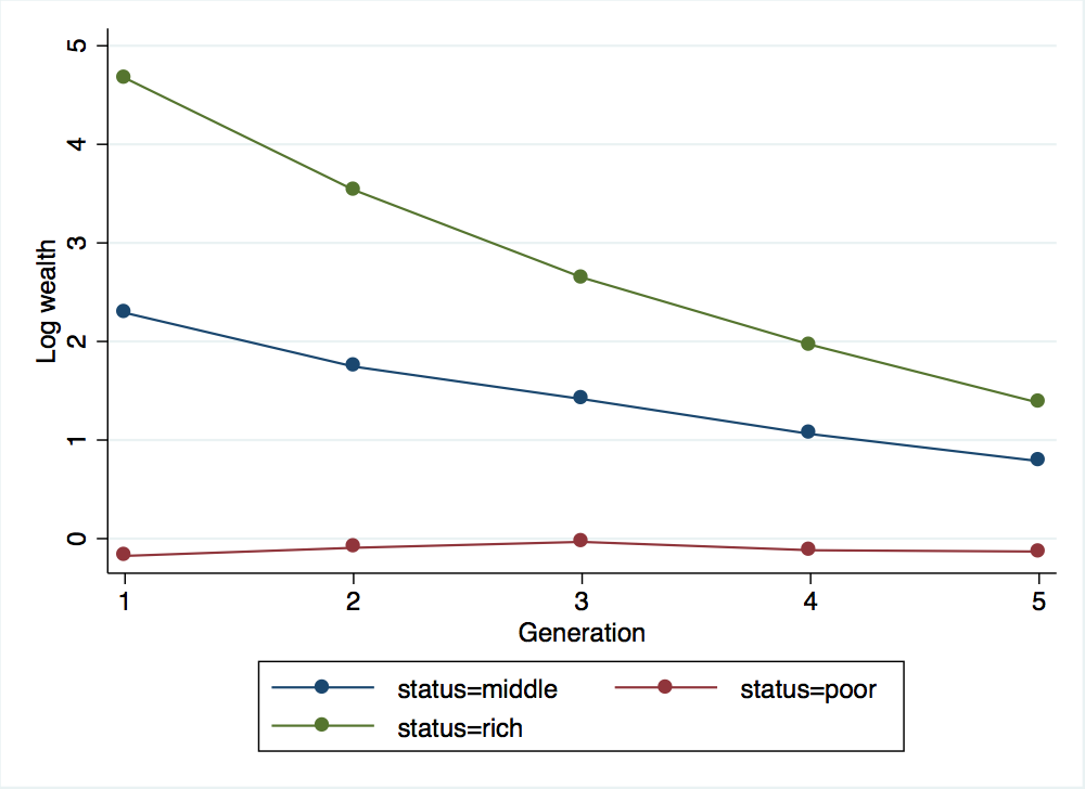
The graphs for these three different values of \(\sigma_{x}\) all look quite similar. From the graphs, you would be inclined to say that all three scenarios exhibit roughly the same degree of intergenerational mobility and the same rate of reversion to the mean. However, the regressions from each scenario give dramatically different values for \(\hat{\beta}\), with lower values of \(\sigma_{x}\) leading to much lower estimates of \(\beta\). This is exactly the point that Clark and Cummins are highlighting in their paper: looking at the correlation in wealth between just two generations can lead to you to severely overestimate the rate at which wealth levels will converge, particularly when the random component of wealth is quite large relative to the variance in the underlying social status transmitted from one generation to the next.