28 February 2018
I have pulled demographic and educational attainment data from the IPUMS one percent samples of the 1880, 1900, 1920 and 1940 federal censuses. The resulting dataset is available here. We will use these data to explore age heaping, the tendency to round ages to particular numbers. The most common numbers to round to are those ending in zero or five.
First things first, let’s load the data and construct a variable that gives us the last digit of each individual’s age:
. clear

. use ipums-sample-for-age-heaping.dta

. gen last_digit = mod(age,10)
The mod function gives the modulus of the first number with respect to the second number. In other words, it gives you the remainder after dividing the first number by the second number. By choosing 10 as the second number, the mod function is effectively giving us the last digit of age.
The last digit of age should be distributed fairly uniformly, we do not expect any real cyclicality of births relative to census years. So if people are correctly reporting their ages, we would expect roughly the same number of people to have an age ending in zero, one, two, three and so on. However, this will not necessarily be true at very young ages and very old ages where mortality is an issue. Particularly in the earlier census years, childhood mortality is still a big issue. A significant number child deaths occur at early ages. So there will be more one-year-olds than two-year-olds and more two-year-olds than three-year-olds even if the same number of children are born each year. The same goes for the elderly, many of the people that make it to age 70 will not make it to age 71, many that make it to 71 will not make it to 72 and so on. So for the very young and the very old, we do not expect a uniform distribution of the last digit for age. Instead, lower digits should be more likely than higher digits. Let’s check this really quickly:
. tab last_digit if year==1880 & age<10

 last_digit │      Freq.     Percent        Cum.
────────────┼───────────────────────────────────
          0 │     14,510       10.78       10.78
          1 │     12,788        9.50       20.27
          2 │     14,377       10.68       30.95
          3 │     13,966       10.37       41.32
          4 │     14,076       10.45       51.78
          5 │     13,598       10.10       61.88
          6 │     13,718       10.19       72.07
          7 │     13,063        9.70       81.77
          8 │     12,898        9.58       91.35
          9 │     11,652        8.65      100.00
────────────┼───────────────────────────────────
      Total │    134,646      100.00

. tab last_digit if year==1880 & age>59

 last_digit │      Freq.     Percent        Cum.
────────────┼───────────────────────────────────
          0 │      6,931       24.30       24.30
          1 │      2,457        8.61       32.91
          2 │      3,158       11.07       43.98
          3 │      2,808        9.84       53.82
          4 │      2,517        8.82       62.64
          5 │      3,406       11.94       74.58
          6 │      2,035        7.13       81.72
          7 │      1,775        6.22       87.94
          8 │      1,904        6.67       94.61
          9 │      1,537        5.39      100.00
────────────┼───────────────────────────────────
      Total │     28,528      100.00
So in 1880, it looks like mortality is affecting the distribution of last digits, particularly for the elderly. Let’s see if this changes by 1940 when medical technology is much better:
. tab last_digit if year==1940 & age<10

 last_digit │      Freq.     Percent        Cum.
────────────┼───────────────────────────────────
          0 │     19,179        8.55        8.55
          1 │     21,692        9.67       18.21
          2 │     23,161       10.32       28.53
          3 │     22,381        9.97       38.50
          4 │     22,808       10.16       48.66
          5 │     22,961       10.23       58.89
          6 │     22,051        9.82       68.72
          7 │     22,563       10.05       78.77
          8 │     23,870       10.64       89.41
          9 │     23,772       10.59      100.00
────────────┼───────────────────────────────────
      Total │    224,438      100.00

. tab last_digit if year==1940 & age>59

 last_digit │      Freq.     Percent        Cum.
────────────┼───────────────────────────────────
          0 │     21,822       15.94       15.94
          1 │     14,320       10.46       26.39
          2 │     16,213       11.84       38.23
          3 │     14,707       10.74       48.97
          4 │     14,027       10.24       59.22
          5 │     15,084       11.02       70.23
          6 │     10,992        8.03       78.26
          7 │     10,570        7.72       85.98
          8 │     10,216        7.46       93.44
          9 │      8,983        6.56      100.00
────────────┼───────────────────────────────────
      Total │    136,934      100.00
By 1940, we do not really see a systematic trend in the frequency of last digits among children but we still see a noticeable downward trend for the elderly. This should make sense. Improvements in health at the turn of the century made a big difference for infants and children but deaths at old ages are always going to be present.
Let’s ignore the deaths at very young and very old ages, focusing our attention on people between the ages of 20 and 59. Within this range, it is reasonable to assume that the last digit of age should be fairly uniformly distributed. Let’s check:
. tab last_digit if age>19 & age<60

 last_digit │      Freq.     Percent        Cum.
────────────┼───────────────────────────────────
          0 │    243,892       12.94       12.94
          1 │    177,709        9.43       22.38
          2 │    204,582       10.86       33.23
          3 │    185,421        9.84       43.07
          4 │    184,922        9.81       52.89
          5 │    204,573       10.86       63.74
          6 │    177,017        9.39       73.14
          7 │    165,788        8.80       81.94
          8 │    178,544        9.48       91.41
          9 │    161,788        8.59      100.00
────────────┼───────────────────────────────────
      Total │  1,884,236      100.00
This looks pretty uniform except for one unusual feature. There appears to be far too many people with ages ending in zero (and a few too many with ages ending in five) than we would expect. This prominence of zeros and, to a lesser extent, fives suggests that there may be age heaping taking place. Of course, it could be the case that there really are many more 20, 30, 40, and 50 year olds than 21, 31, 41 and 51 year olds. How can we check whether this is the true distribution of ages or whether there is rounding?
We cannot know for certain, but we can make some assumptions about how the likelihood of heaping should correspond to other individual characteristics. In particular, let’s assume that people with lower levels of human capital are more likely to round their ages. We can use the data to test whether people with ages ending in zero or five are more educated or less educated on average than people with ages ending in other digits. To do this, we will start by constructing an indicator variable equal to one if an individual has an age ending in zero or five and equal to zero otherwise. To measure human capital, we will construct an indicator for literacy, an indicator for being a high school graduate, and a measure of years of schooling:
. gen zero_or_five = 0 if last_digit~=0 & last_digit~=5
(833,278 missing values generated)

. replace zero_or_five = 1 if last_digit==0 | last_digit==5
(833,278 real changes made)

. gen literate = 0 if lit==1
(3,511,419 missing values generated)

. replace literate = 1 if lit==2 | lit==3 | lit==4
(1,616,129 real changes made)

. gen years_of_schooling = 0 if higrade==1
(3,481,606 missing values generated)

. replace years_of_schooling = higrade - 3 if higrade>1 & higrade~=.
(1,168,072 real changes made)

. gen hs_grad = 0 if years_of_schooling < 12 & years_of_schooling~=.
(2,570,058 missing values generated)

. replace hs_grad = 1 if years_of_schooling > 11 & years_of_schooling~=.
(256,524 real changes made)
Now we can run some simple regressions to see if these measures of human capital help us predict having an age ending in zero or five:
. reg zero_or_five literate if age>19 & age<60

      Source │       SS           df       MS      Number of obs   = 1,150,044
─────────────┼──────────────────────────────────   F(1, 1150042)   =   4539.90
       Model │  841.535029         1  841.535029   Prob > F        =    0.0000
    Residual │  213176.744 1,150,042  .185364312   R-squared       =    0.0039
─────────────┼──────────────────────────────────   Adj R-squared   =    0.0039
       Total │  214018.279 1,150,043  .186095893   Root MSE        =    .43054

─────────────┬────────────────────────────────────────────────────────────────
zero_or_five │      Coef.   Std. Err.      t    P>|t|     [95% Conf. Interval]
─────────────┼────────────────────────────────────────────────────────────────
    literate │  -.0956001   .0014188   -67.38   0.000     -.098381   -.0928192
       _cons │   .3344165   .0013552   246.77   0.000     .3317605    .3370726
─────────────┴────────────────────────────────────────────────────────────────

. reg zero_or_five hs_grad if age>19 & age<60

      Source │       SS           df       MS      Number of obs   =   734,192
─────────────┼──────────────────────────────────   F(1, 734190)    =     73.24
       Model │  12.7133561         1  12.7133561   Prob > F        =    0.0000
    Residual │  127445.619   734,190    .1735867   R-squared       =    0.0001
─────────────┼──────────────────────────────────   Adj R-squared   =    0.0001
       Total │  127458.333   734,191   .17360378   Root MSE        =    .41664

─────────────┬────────────────────────────────────────────────────────────────
zero_or_five │      Coef.   Std. Err.      t    P>|t|     [95% Conf. Interval]
─────────────┼────────────────────────────────────────────────────────────────
     hs_grad │   .0091517   .0010694     8.56   0.000     .0070558    .0112477
       _cons │   .2209283   .0005779   382.30   0.000     .2197957     .222061
─────────────┴────────────────────────────────────────────────────────────────

. reg zero_or_five years_of_schooling if age>19 & age<60

      Source │       SS           df       MS      Number of obs   =   734,192
─────────────┼──────────────────────────────────   F(1, 734190)    =      0.05
       Model │  .009526401         1  .009526401   Prob > F        =    0.8148
    Residual │  127458.323   734,190  .173604003   R-squared       =    0.0000
─────────────┼──────────────────────────────────   Adj R-squared   =   -0.0000
       Total │  127458.333   734,191   .17360378   Root MSE        =    .41666

───────────────────┬────────────────────────────────────────────────────────────────
      zero_or_five │      Coef.   Std. Err.      t    P>|t|     [95% Conf. Interval]
───────────────────┼────────────────────────────────────────────────────────────────
years_of_schooling │   -.000032   .0001367    -0.23   0.815       -.0003    .0002359
             _cons │    .223886   .0013106   170.82   0.000     .2213172    .2264548
───────────────────┴────────────────────────────────────────────────────────────────
Let’s do this a little more systematically, including additional potentially relevant controls.
. gen black = 0

. replace black = 1 if race==2
(395,115 real changes made)

. gen female = 0

. replace female = 1 if sex==2
(1,806,991 real changes made)

. reg zero_or_five literate black female

      Source │       SS           df       MS      Number of obs   = 1,769,976
─────────────┼──────────────────────────────────   F(3, 1769972)   =   3006.96
       Model │  1644.62128         3  548.207094   Prob > F        =    0.0000
    Residual │  322688.174 1,769,972  .182312587   R-squared       =    0.0051
─────────────┼──────────────────────────────────   Adj R-squared   =    0.0051
       Total │  324332.795 1,769,975  .183241455   Root MSE        =    .42698

─────────────┬────────────────────────────────────────────────────────────────
zero_or_five │      Coef.   Std. Err.      t    P>|t|     [95% Conf. Interval]
─────────────┼────────────────────────────────────────────────────────────────
    literate │  -.0792631   .0012291   -64.49   0.000    -.0816722   -.0768541
       black │   .0449308   .0011236    39.99   0.000     .0427285    .0471332
      female │   .0045789   .0006421     7.13   0.000     .0033204    .0058374
       _cons │   .3069861   .0012561   244.39   0.000     .3045241    .3094481
─────────────┴────────────────────────────────────────────────────────────────
Finally, let’s add some fixed effects for region and census year:
. xi: reg zero_or_five literate black female i.region i.year
i.region          _Iregion_11-91      (naturally coded; _Iregion_11 omitted)
i.year            _Iyear_1880-1940    (naturally coded; _Iyear_1880 omitted)
note: _Iyear_1940 omitted because of collinearity

      Source │       SS           df       MS      Number of obs   = 1,769,976
─────────────┼──────────────────────────────────   F(14, 1769961)  =    773.55
       Model │  1972.40261        14  140.885901   Prob > F        =    0.0000
    Residual │  322360.392 1,769,961  .182128528   R-squared       =    0.0061
─────────────┼──────────────────────────────────   Adj R-squared   =    0.0061
       Total │  324332.795 1,769,975  .183241455   Root MSE        =    .42677

─────────────┬────────────────────────────────────────────────────────────────
zero_or_five │      Coef.   Std. Err.      t    P>|t|     [95% Conf. Interval]
─────────────┼────────────────────────────────────────────────────────────────
    literate │  -.0744088   .0012435   -59.84   0.000     -.076846   -.0719716
       black │   .0460044   .0012098    38.03   0.000     .0436332    .0483757
      female │   .0044168   .0006423     6.88   0.000     .0031578    .0056758
 _Iregion_12 │   .0022653   .0013544     1.67   0.094    -.0003892    .0049198
 _Iregion_21 │  -.0102248   .0013531    -7.56   0.000    -.0128769   -.0075728
 _Iregion_22 │  -.0111654   .0014748    -7.57   0.000     -.014056   -.0082748
 _Iregion_31 │  -.0009243   .0015087    -0.61   0.540    -.0038813    .0020327
 _Iregion_32 │  -.0093862   .0016187    -5.80   0.000    -.0125589   -.0062136
 _Iregion_33 │  -.0102054   .0016365    -6.24   0.000    -.0134128    -.006998
 _Iregion_41 │   .0000999   .0023554     0.04   0.966    -.0045167    .0047165
 _Iregion_42 │    .000526    .001924     0.27   0.785     -.003245    .0042971
 _Iregion_91 │  -.0386298   .0137706    -2.81   0.005    -.0656197   -.0116399
 _Iyear_1900 │  -.0266067   .0009017   -29.51   0.000     -.028374   -.0248393
 _Iyear_1920 │  -.0324146    .000855   -37.91   0.000    -.0340905   -.0307388
 _Iyear_1940 │          0  (omitted)
       _cons │    .331187   .0017642   187.73   0.000     .3277292    .3346447
─────────────┴────────────────────────────────────────────────────────────────
These regressions seem to confirm that there is likely rounding taking place. Zeros and fives are substantially more common among illiterate individuals, among black individuals relative to white individuals, and in 1880 relative to the more recent census years.
In the literature on age heaping, a few different measures are used to describe the extent of heaping, or rounding, in the sample. One simple measure is the following heaping index:
\[\begin{equation} H_{i} = \frac{5}{4} \left( X_{i} - 20\right) \end{equation}\]\(X_{i}\) is the proportion of individuals in sample \(i\) with an age ending in either zero or five, expressed as a percentage. \(H_{i}\) then ranges from zero in the case of no heaping (20 percent of individuals have an age ending in zero or five) to 100 (100 percent of individuals have an age ending in zero or five). Let’s go ahead and calculate this heaping index at the state-race-year level using the collapse command:
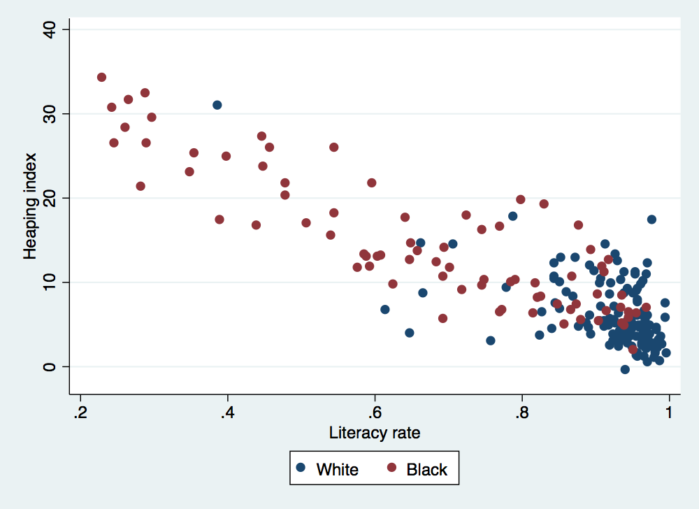
. keep if age>19 & age<60
(1,781,030 observations deleted)

. collapse (sum) rounded_sum = zero_or_five (count) all_sum = zero_or_five (mean) mean_literacy_rate = literate, by(stateicp
> black year)

. gen heaping_index = (5/4) * ( 100 * rounded_sum/all_sum - 20)

. twoway (scatter heaping_index mean_literacy_rate if black==0 & all_sum>100) (scatter heaping_index mean_literacy_rate if bl
> ack==1 & all_sum>100), ytitle(Heaping index) xtitle(Literacy rate) legend(order(1 "White" 2 "Black"))

. graph export heaping-v-literacy.png, width(500) replace
(file heaping-v-literacy.png written in PNG format)
That is a pretty clear negative relationship at the state level between age heaping and literacy.
A couple of quick notes about the graphing command above. Notice that I restricted the plot to states with at least 100 individuals used to calculated the heaping index. When there are a small number of individuals, any index like the heaping index will become quite noisy and rather uninformative (you can take a look at just how ugly the graph gets for yourself if you drop the restriction on the all_sum variable). Also note that I changed the keys for the legend. Unless you do a good job of nicely labeling the values of your variables, you will typically end up with pretty uninformative legends.
In class, we saw a slightly different approach to age heaping used by Ó’Gráda and Mokyr. They estimated the following measure of age heaping: \[\begin{equation} \gamma = \sum_{i=15}^{34} \left( \frac{n_{i}}{\sum{n_{i}}} - \frac{\hat{n_{i}}}{\sum\hat{n_{i}}}\right)^{2} \end{equation}\] where \(n_{i}\) is the observed number of people of age \(i\) and \(\hat{n_{i}}\) is the predicted number based on a smooth polynomial. Try implementing this alternative definition of age heaping using a quartic polynomial to get the predicted \(\hat{n_{i}}\) values.
In theory, the original dataset contains the same individuals at multiple points in time (in practice, these are based on one percent sample so it is very unlikely the same individual appears twice). This gives us a chance to see whether people round ages more or less as they get older. For the cohort born between 1860 and 1870, determine whether age heaping is getting more or less pronounced as they get older.
For young children, we would not expect to see ages getting rounded to zero or five; the difference between 43 and 45 is a whole lot smaller than the difference between 3 and 5. However, that does not mean ages are being accurately reported for young children. Can you detect any patterns that suggest rounding of ages for children under the age of 10 in the census?
One other reason for misreporting age is that various laws have age cutoffs. For example, under current laws you must be 18 to vote and 21 to purchase alcohol. If you asked for ages on a college campus, you might find the number of people stating they are 21 to be curiously higher than the number of people stating they are 20. What ages might people falsely claim in these census samples (1880, 1900, 1920, 1940)? Do you see evidence that individuals are falsely claiming these ages?