24 September 2019
First, let’s construct a sample of fathers and sons, matching certains characteristics of the joint distribution of father and son earnings in the United States. We will start by generated a sample of 10,000 fathers whose incomes are distributed log normally with a mean and standard deviation equal to that given in the sample if Solon (1992).
. clear

. set obs 5000
number of observations (_N) was 0, now 5,000

. gen id = _n

. set seed 24892217
The set obs command generates an empty 5,000 observation dataset. The gen id command simply creates a unique id number for each observation equal to its observation number. Finally, the set seed specifies the seed for Stata’s random number generator. (Note: I am setting the seed solely so that the same results get generated each time I compile this document. I chose the seed number based on the serial number of a bill in my pocket).
Now we are going to generate fathers’ incomes assuming that earnings are distributed log normal. We can do this by creating log income as a random variable using Stata’s rnormal function, using the mean and standard deviation from Table 1 in Solon (1992).
. gen log_father_inc = rnormal(10.1,0.69)
As for sons’ earnings, we would like those to be a function of fathers’ earnings. We will assume that sons’ log earnings are linearly related to fathers’ log earnings with a mean zero, normally distributed error term:
The value of β1 can be taken directly from the estimated coefficient in Table 2 of Solon (1992). The value of β0 is then simply equal to the mean log income for sons in Table 1 minus β1 times the mean log income for fathers in Table 1. Finally, we can choose the standard deviation for ε that, once used in the above equation, generates son incomes that match the standard deviation of log son earnings given in Table 1. This leads to a value of 0.413 for β1, 5.58 for β0 and 0.94 for σε. With these values, we can now generate sons’ log income values:
. gen son_epsilon = rnormal(0,0.94)

. gen log_son_inc = 5.58+.413 * log_father_inc + son_epsilon

. gen father_inc = exp(log_father_inc)

. gen son_inc = exp(log_son_inc)
Let’s take a quick look at our generated incomes, summarizing the data, looking at the correlation between father and son incomes, and then looking at the income distributions graphically.
. sum log_son_inc log_father_inc
Variable │ Obs Mean Std. Dev. Min Max
─────────────┼─────────────────────────────────────────────────────────
log_son_inc │ 5,000 9.758711 .9891708 6.166673 13.89211
log_father~c │ 5,000 10.09548 .6920174 7.581927 12.72381
. corr log_son_inc log_father_inc
(obs=5,000)
│ log_so~c log_fa~c
─────────────┼──────────────────
log_son_inc │ 1.0000
log_father~c │ 0.3022 1.0000
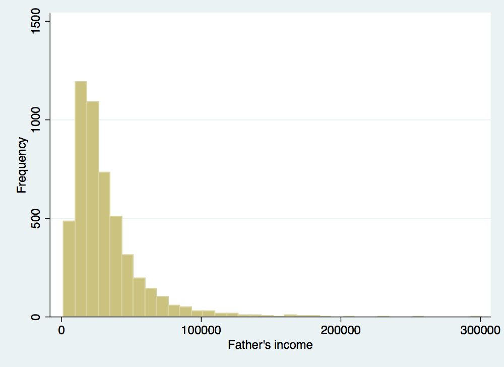
. histogram father_inc, frequency ytitle(Frequency) xtitle(Father's income)
(bin=36, start=1962.4065, width=9268.9957)
. graph export father_inc.png, width(500) replace
(file father_inc.png written in PNG format)
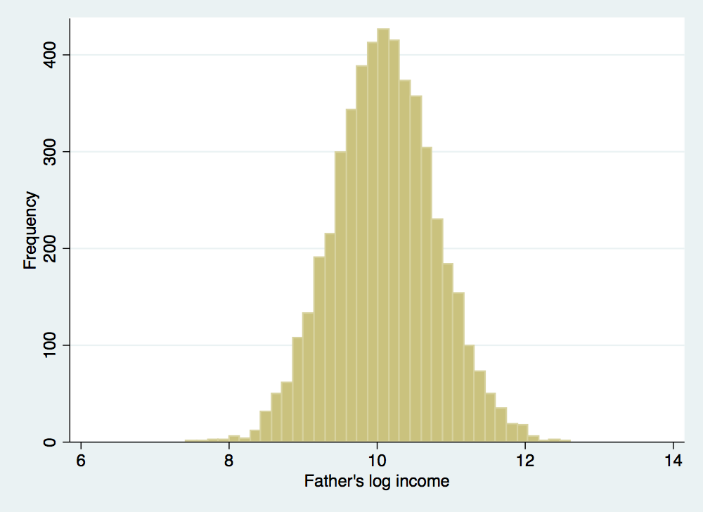
. histogram log_father_inc, frequency ytitle(Frequency) xtitle(Father's log income)
(bin=36, start=7.5819268, width=.14283017)
. graph export log_father_inc.png, width(500) replace
(file log_father_inc.png written in PNG format)
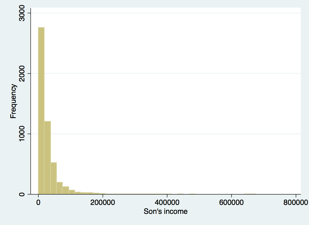
. histogram son_inc, frequency ytitle(Frequency) xtitle(Son's income)
(bin=36, start=476.5979, width=29975.997)
. graph export son_inc.png, width(500) replace
(file son_inc.png written in PNG format)
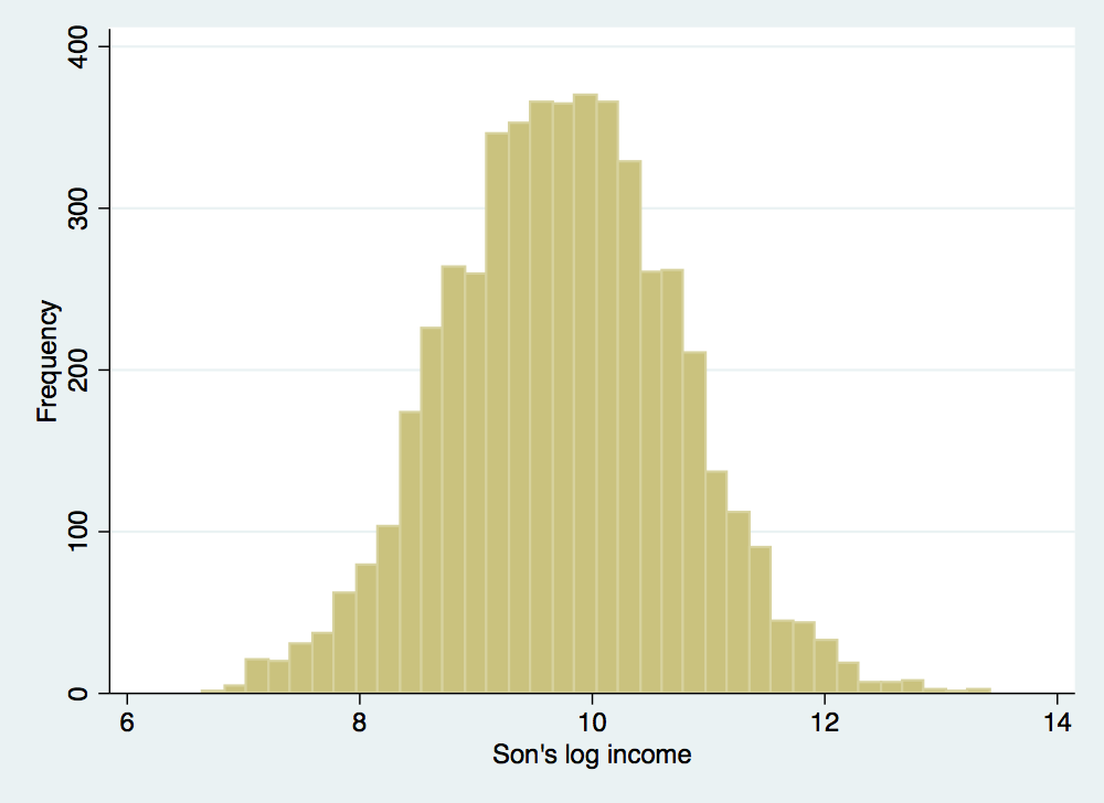
. histogram log_son_inc, frequency ytitle(Frequency) xtitle(Son's log income)
(bin=36, start=6.1666732, width=.21459554)
. graph export log_son_inc.png, width(500) replace
(file log_son_inc.png written in PNG format)
To take a graphical look at the relationship between father and son log incomes, we could use a standard scatterplot. However, with 5,000 observations, a scatterplot will be somewhat uninformative (go ahead and try it yourself using Stata’s scatter command if you would like to see why). Instead, we can use a package for Stata to create a binned scatterplot:
. binscatter log_son_inc log_father_inc, xtitle("Father's log income") ytitle("Son's log income")

. graph export father_son_scatter.png, width(500) replace
(file father_son_scatter.png written in PNG format)
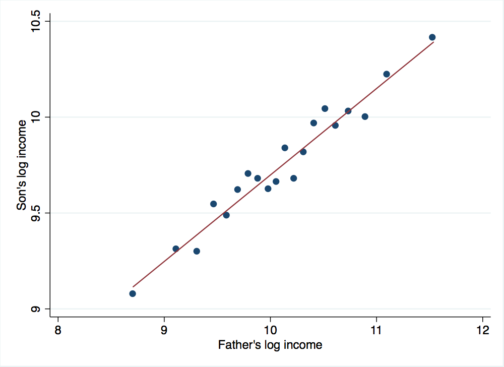
Notice the nice, linear relationship between son’s log income and father’s log income. This should not come as a surprise given that this is how we constructed son’s log income in the first place. If you would like to use the binscatter program on your own computer, you can install it with the following command: ssc install binscatter.
First let’s confirm that our simulated data match the real data used in Solon (1992). To check, let’s run a regression to recover the intergenerational income elasticity for the sample:
. reg log_son_inc log_father_inc

      Source │       SS           df       MS      Number of obs   =     5,000
─────────────┼──────────────────────────────────   F(1, 4998)      =    502.46
       Model │  446.814043         1  446.814043   Prob > F        =    0.0000
    Residual │  4444.50226     4,998  .889256155   R-squared       =    0.0913
─────────────┼──────────────────────────────────   Adj R-squared   =    0.0912
       Total │  4891.31631     4,999  .978458953   Root MSE        =      .943

───────────────┬────────────────────────────────────────────────────────────────
   log_son_inc │      Coef.   Std. Err.      t    P>|t|     [95% Conf. Interval]
───────────────┼────────────────────────────────────────────────────────────────
log_father_inc │    .432021   .0192732    22.42   0.000      .394237     .469805
         _cons │   5.397252   .1950292    27.67   0.000     5.014909    5.779595
───────────────┴────────────────────────────────────────────────────────────────
From the regression results, we see that we get a coefficient on father’s log income 0.43. Thus we have an intergenerational income elasticity (roughly) equal to that of Solon (1992). We can think of this as the true intergenerational income elasticity for our sample. Now we will consider what happens with two common problems with the way incomes are recorded in survey data: rounding and censoring.
First, we will explore the effects of rounding. Suppose that the survey provides options for income that are in $5,000 intervals (alternatively, assume that people tend to round their incomes to the nearest $5,000). We can generate rounded versions of the father and son incomes using Stata’s round function and then take the natural log to get rounded log income values:
. gen rounded_father_inc = round(father_inc,5000)

. gen rounded_son_inc = round(son_inc,5000)

. gen log_rounded_father_inc = ln(rounded_father_inc)
(4 missing values generated)

. gen log_rounded_son_inc = ln(rounded_son_inc)
(121 missing values generated)
Now we can use these new variables to re-estimate our intergenerational income elasticity:
. reg log_rounded_son_inc log_rounded_father_inc

      Source │       SS           df       MS      Number of obs   =     4,876
─────────────┼──────────────────────────────────   F(1, 4874)      =    418.22
       Model │  321.010598         1  321.010598   Prob > F        =    0.0000
    Residual │  3741.14468     4,874  .767571743   R-squared       =    0.0790
─────────────┼──────────────────────────────────   Adj R-squared   =    0.0788
       Total │  4062.15527     4,875   .83326262   Root MSE        =    .87611

───────────────────────┬────────────────────────────────────────────────────────────────
   log_rounded_son_inc │      Coef.   Std. Err.      t    P>|t|     [95% Conf. Interval]
───────────────────────┼────────────────────────────────────────────────────────────────
log_rounded_father_inc │   .3714719   .0181646    20.45   0.000     .3358611    .4070826
                 _cons │   6.073227   .1839989    33.01   0.000     5.712506    6.433947
───────────────────────┴────────────────────────────────────────────────────────────────
Notice that the measurement error we introduced by rounding incomes has led to an attenuation bias for the intergenerational income elasticity, substantially reducing the estimated coefficient on father’s log income to 0.37. Using rounded incomes, without acknowledging the impact of this rounding on the estimation, would lead us to conclude there is significantly more income mobility than is actually in the underlying data.
The rounding exercise also demonstrates another problem. If you look closely at the commands generating new log incomes, you will notice that several missing values were generated. These missing values are cases where the income was rounded to zero and the natural log of zero does not exist, hence the missing value for log income. One criticism of the intergenerational income elasticity is that its calculation requires dropping individuals with no earnings.
Now we will consider what happens when we top code incomes, a common practice in income datasets. We will impose a top code of $100,000 in our dataset using Stata’s min function (all incomes above $100,000 simply get coded as $100,000):
. gen censored_father_inc = min(rounded_father_inc,100000)

. gen censored_son_inc = min(rounded_son_inc,100000)

. gen log_censored_father_inc = ln(censored_father_inc)
(4 missing values generated)

. gen log_censored_son_inc = ln(censored_son_inc)
(121 missing values generated)

. reg log_censored_son_inc log_censored_father_inc

      Source │       SS           df       MS      Number of obs   =     4,876
─────────────┼──────────────────────────────────   F(1, 4874)      =    413.22
       Model │  296.981315         1  296.981315   Prob > F        =    0.0000
    Residual │  3502.90966     4,874  .718692995   R-squared       =    0.0782
─────────────┼──────────────────────────────────   Adj R-squared   =    0.0780
       Total │  3799.89097     4,875  .779464815   Root MSE        =    .84776

────────────────────────┬────────────────────────────────────────────────────────────────
   log_censored_son_inc │      Coef.   Std. Err.      t    P>|t|     [95% Conf. Interval]
────────────────────────┼────────────────────────────────────────────────────────────────
log_censored_father_inc │   .3635857    .017886    20.33   0.000      .328521    .3986504
                  _cons │   6.141692   .1810735    33.92   0.000     5.786706    6.496678
────────────────────────┴────────────────────────────────────────────────────────────────
Notice that this further reduces our estimated intergenerational income elasticity to 0.36. The main takeaway is the same, whether we introduce mismeasurement through rounding or censoring of the data, any mismeasurement leads to the appearance of a weaker relationship between father and son’s incomes. This leads to a lower estimated intergenerational income elasticity, leading us to the false conclusion that there is greater mobility. However, this greater estimated mobility is simply the product of measurement, it has nothing to do with sons’ fortunes being less closely tied to those of their fathers.
Now we will turn our attention to the difference between average income over the life cycle and income in the current period. In general, annual income over the life cycle follows a concave shape, with earnings rising over the early career of an individual and then falling in the final years of the career. This suggests that observing earnings very early or very late in an individual’s career will lead to underestimates of average earnings and observing earnings in the peak of a career will lead to overestimates of average earnings. This problem can be handled reasonably well by controlling for a quadratic in an individual’s age.
More problematic is that individuals experience transitory fluctuations in income over their careers, temporary rises and falls in income unrelated to overall trends over the life cycle. To examine the effect these transitory fluctuations have on the estimated income elasticity, let’s introduce some random ups and downs in father and son’s earnings. We can introduce these transitory fluctuations by treating our son_inc and father_inc variables as our average lifetime annual income and creating a new observation of annual income that includes a random increase or decrease relative to this average income.
. gen father_income_shock = (runiform()-.5)

. gen transitory_father_inc = father_inc * (1+father_income_shock)

. gen log_transitory_father_inc = ln(transitory_father_inc)

. gen son_income_shock = (runiform()-.5)

. gen transitory_son_inc = son_inc * (1+son_income_shock)

. gen log_transitory_son_inc = ln(transitory_son_inc)
In the above commands, we have adjusted incomes by a random percentage ranging with a uniform probability between negative 50% and positive 50%. We can think of these new incomes as observations of a single year of income and the original income variables as observations of the true lifetime average annual income. Now we can see the impact of using one year’s earnings rather than average annual earnings on our estimate of intergenerational income elasticity:
. reg log_transitory_son_inc log_transitory_father_inc

      Source │       SS           df       MS      Number of obs   =     5,000
─────────────┼──────────────────────────────────   F(1, 4998)      =    375.64
       Model │   378.21947         1   378.21947   Prob > F        =    0.0000
    Residual │  5032.31492     4,998  1.00686573   R-squared       =    0.0699
─────────────┼──────────────────────────────────   Adj R-squared   =    0.0697
       Total │  5410.53439     4,999  1.08232334   Root MSE        =    1.0034

──────────────────────────┬────────────────────────────────────────────────────────────────
   log_transitory_son_inc │      Coef.   Std. Err.      t    P>|t|     [95% Conf. Interval]
──────────────────────────┼────────────────────────────────────────────────────────────────
log_transitory_father_inc │   .3632171   .0187405    19.38   0.000     .3264776    .3999566
                    _cons │   6.063303   .1888758    32.10   0.000     5.693024    6.433583
──────────────────────────┴────────────────────────────────────────────────────────────────
Our estimated intergenerational elasticity is now reduced to 0.36, a rather substantial attenuation bias that would lead us to overestimate the extent of intergenerational mobility. For how transitory fluctuations impact real data, consider Table 2 in Solon (1992), our source for our empirical elasticity estimate. The estimates in this table demonstrate a clear increase in estimated intergenerational income elasticities as more periods are used to construct average incomes. In a more recent example, Mazumder (2005) finds large changes in the intergenerational income elasticity when using a single observation of annual income versus an average of several years of annual income observations (see Figure 4). One important difference is that our random income shocks may be a bit different than real world random income shocks. In particular, Mazumder notes that transitory income shocks may exhibit some persistence. This autocorrelation in real-world transitory shocks will further weaken the association between father and son incomes, creating a greater attenuation of the intergenerational income elasticity estimate.