25 September 2019
For the first part of this exercise, we will be using the Stata data file us-wid-data.dta. This file is based on the data available through the World Wealth and Income Database. To generate the data set, I used the following commands in Stata:
For the second part of this exercise, we will use data from the Integrated Public Use Microdata Series. IPUMS provides an incredibly convenient interface for downloading samples of historical federal census data as well as a wide range of other datasets. There are two different datasets that I constructed through IPUMS: 1870-census-wealth-data.dta and 1940-census-income-data.dta. Both of these are available on the course website. You can create your own census extracts using the IPUMS website after creating a free account.
Now let’s go ahead and get started by opening the WID data file. When we open it, we will first clear out Stata’s memory just in case a file is already open:
. clear

. use us-wid-data.dta
If you are working on your own computer, the WID package is the easiest way to get the wealth and income data in Stata. If you are on a campus computer, Stata will not let you install the package. Instead, you can download a copy of the us-wid-data.dta file from our course website. If you would like additional variables or data from other countries, you can also use the data download tools on the WID website to generate your own samples.
Before we can work with the data, it will be useful to reshape the data. Let’s list the data for a single year to look at the current structure of the dataset:
. list if year == 1980

      ┌──────────────────────────────────────────────────┐
      │ country     variable   percen~e   year     value │
      ├──────────────────────────────────────────────────┤
  17. │      US   shweal992j       p0p1   1980   -.00423 │
  68. │      US   shweal992j      p0p10   1980   -.01058 │
 121. │      US   shweal992j      p0p50   1980    .01055 │
 172. │      US   shweal992j    p50p100   1980    .98939 │
 223. │      US   shweal992j    p75p100   1980    .87975 │
      ├──────────────────────────────────────────────────┤
 325. │      US   shweal992j    p90p100   1980    .65102 │
 427. │      US   shweal992j    p95p100   1980    .49045 │
 529. │      US   shweal992j    p99p100   1980    .23554 │
 580. │      US   sptinc992j       p0p1   1980   -.00033 │
 631. │      US   sptinc992j      p0p10   1980     .0102 │
      ├──────────────────────────────────────────────────┤
 684. │      US   sptinc992j      p0p50   1980    .19894 │
 735. │      US   sptinc992j    p50p100   1980     .8011 │
 786. │      US   sptinc992j    p75p100   1980    .56004 │
 888. │      US   sptinc992j    p90p100   1980    .34243 │
 990. │      US   sptinc992j    p95p100   1980    .23904 │
      ├──────────────────────────────────────────────────┤
1092. │      US   sptinc992j    p99p100   1980    .10671 │
      └──────────────────────────────────────────────────┘
Notice that each year has multiple observations, one for each of our key income or wealth variables. This is what Stata refers to as data in long format. We would prefer to have one observation per year with all of the income and wealth variables included, this will let us easily compare values over time (for example, graphing how both the bottom decile and top decile shares of income evolve over time). This is called data in wide format. Stata’s reshape command converts between long and wide format. Before we use it, let’s restrict our data to just one of the outcomes (wealth share or income share) to make it a bit simpler to see what is going on:
. keep if variable == "shweal992j"
(563 observations deleted)

. rename value wealth

. reshape wide wealth, i(year) j(percentile) string
(note: j = p0p1 p0p10 p0p50 p50p100 p75p100 p90p100 p95p100 p99p100)

Data                               long   ->   wide
─────────────────────────────────────────────────────────────────────────────
Number of obs.                      563   ->     102
Number of variables                   5   ->      11
j variable (8 values)        percentile   ->   (dropped)
xij variables:
                                 wealth   ->   wealthp0p1 wealthp0p10 ... wealthp99p100
─────────────────────────────────────────────────────────────────────────────
Now we can see what the new format of the data looks like:
. list if year == 1980

     ┌─────────────────────────────────────────────────────────────────────────────────────────────────────────────────────┐
     │ year   wealth~1   wealt~10   wealt~50   w~50p100   w~75p100   w~90p100   w~95p100   we~9p100   country     variable │
     ├─────────────────────────────────────────────────────────────────────────────────────────────────────────────────────┤
 68. │ 1980    -.00423    -.01058     .01055     .98939     .87975     .65102     .49045     .23554        US   shweal992j │
     └─────────────────────────────────────────────────────────────────────────────────────────────────────────────────────┘
Notice that all of the wealth percentiles for a given year are now included in a single observation. Also notice that Stata has created new variable names for us, combining the name of our key variable for reshaping, wealth, with the value of our j variable, percentile in this case. This makes it much easier to compare two different parts of the distribution over time. For example, let’s just list the shares for bottom and top halves of the distribution for the 1990s:
. list year wealthp0p50 wealthp50p100 if year>1989 & year<2000

     ┌─────────────────────────────┐
     │ year   wealt~50   we~50p100 │
     ├─────────────────────────────┤
 78. │ 1990     .02192      .97807 │
 79. │ 1991      .0215   .97845999 │
 80. │ 1992       .019      .98107 │
 81. │ 1993     .01764      .98234 │
 82. │ 1994     .01575      .98428 │
     ├─────────────────────────────┤
 83. │ 1995     .01367      .98633 │
 84. │ 1996     .01241      .98759 │
 85. │ 1997     .00997   .99005001 │
 86. │ 1998     .00959      .99036 │
 87. │ 1999     .01052      .98951 │
     └─────────────────────────────┘
Much easier than having a separate observation for each outcome in each year.
One downside of keeping only the wealth variable is that we may want to look at wealth and income inequality trends side by side. We can do this by creating a second dataset with income data and then merging the two datasets back together. First, we’ll save our wealth data and then follow the same steps we took above to create an income inequality dataset.
. save us-wealth-data.dta, replace
file us-wealth-data.dta saved

. clear

. use us-wid-data.dta

. keep if variable == "sptinc992j"
(563 observations deleted)

. rename value income

. reshape wide income, i(year) j(percentile) string
(note: j = p0p1 p0p10 p0p50 p50p100 p75p100 p90p100 p95p100 p99p100)

Data                               long   ->   wide
─────────────────────────────────────────────────────────────────────────────
Number of obs.                      563   ->     102
Number of variables                   5   ->      11
j variable (8 values)        percentile   ->   (dropped)
xij variables:
                                 income   ->   incomep0p1 incomep0p10 ... incomep99p100
─────────────────────────────────────────────────────────────────────────────

. save us-income-data.dta, replace
file us-income-data.dta saved
To merge the data, we will use Stata’s merge command. When using this command, we need a variable to merge on. In this case, we want to merge on year, combining the wealth and income data from each file into a single observation per year in a new file. First, we need to sort our data on this merge variable:
. clear

. use us-wealth-data.dta

. sort year

. save us-wealth-data.dta, replace
file us-wealth-data.dta saved

. clear

. use us-income-data.dta

. sort year

. save us-income-data.dta, replace
file us-income-data.dta saved
Now we can issue the merge command. Note that there should be one observation per year in each of the datasets. Therefore, we are doing what is called a one to one merge and using the 1:1 option for the merge command. If we had one dataset with a single observation per year and another dataset with multiple observations per year, we would need to do a one to many merge, using the 1:m option. Let’s merge our data:
. merge 1:1 year using us-wealth-data.dta

    Result                           # of obs.
    ─────────────────────────────────────────
    not matched                             0
    matched                               102  (_merge==3)
    ─────────────────────────────────────────
Notice that we specified the type of merge, the variable we are merging on and the file name we are merging the current dataset with. Stata has created a new variable named _merge that keeps track of merging successes and failures. A value of three indicates an observation that was successfully merged between the two datasets. A value of one indicates an observation from the master dataset (the one originally open) that could not be merged to the using dataset. A value of two indicates an observation from the using dataset that could note be merged to the master dataset.
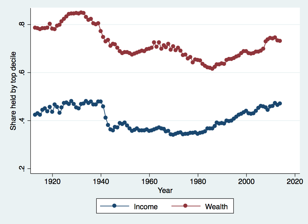
Let’s start by looking at trends in the share of income and wealth held over time by the top decile. To do this, a good approach is to create a twoway graph in Stata. Note that there are many, many options for graphs in Stata and tweaking these options can be very complicated but leads to much better graphs. The easiest approach is to create your first graph from the Graphics menu, selecting all of the various options from the various graphical menus. Once you create the graph, Stata will actually issue the command that includes all of your options. You can copy this command and paste it into a do file so that you can automatically create the same graph or slightly modify the command to tweak the graph appearance without going back through all of the menus.
. twoway (connected incomep90p100 year if year>1900 & year<2020) (connected wealthp90p100 year if year>1900 & year<2020, sort)
> , ytitle(Share held by top decile) xtitle(Year) legend(order(1 "Income" 2 "Wealth"))

. graph export income_and_wealth_over_time.png, width(500) replace
(file income_and_wealth_over_time.png written in PNG format)
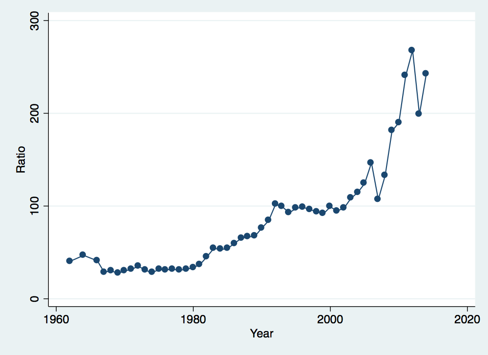
Now let’s construct a ratio of the share of income held by the top decile relative to the share held by the bottom decile and graph its evolution over time.
. gen income_ratio = incomep90p100 / incomep0p10
(51 missing values generated)

. twoway (connected income_ratio year if year>1959 & year<2018), ytitle(Ratio) xtitle(Year) legend(off)

. graph export income_ratio_over_time.png, width(500) replace
(file income_ratio_over_time.png written in PNG format)
What if we worry that this pattern is being driven by the incomes of the top one percent? Let’s get rid of those and see how the pattern changes:
. replace income_ratio = (incomep90p100 - incomep99p100) / incomep0p10
(51 real changes made)

. twoway (connected income_ratio year if year>1959 & year<2018), ytitle(Ratio) xtitle(Year) legend(off)

. graph export income_ratio_over_time_no_top.png, width(500) replace
(file income_ratio_over_time_no_top.png written in PNG format)
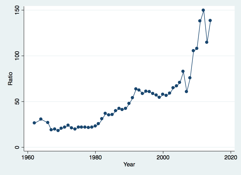
Something very strange has happened. The scale has shifted (the ratios on the vertical axis are now much smaller) but the patterns over time are identical to the previous graph. Is this possible? Think about what we discussed in class about top coding incomes and how that might affect this particular graph.
Take some time to generate your own samples from the WID data to look at more dimensions of wealth and income inequality over time and across countries.
Now let’s switch our attention to the individual-level data available through the federal census. We will start with our 1870 federal census data. The 1870 census is nice for our purposes because it asked individuals to report wealth in terms of both real property and personal property, offering a chance to look at historical wealth distributions as a function of individual demographic characteristics. Let’s load the data:
. clear

. use 1870-census-wealth-data.dta
Our key wealth variables here are realprop and persprop. We also have a proxy for income in the form of occscore, the occupational income score. To see the variable descriptions, we can use the describe command:
. describe realprop persprop occscore

              storage   display    value
variable name   type    format     label      variable label
──────────────────────────────────────────────────────────────────────────────────────────────────────────────────────────────
realprop        long    %12.0g                Real estate value
persprop        long    %12.0g                Value of personal estate
occscore        byte    %8.0g                 Occupational income score

. sum realprop persprop occscore

    Variable │        Obs        Mean    Std. Dev.       Min        Max
─────────────┼─────────────────────────────────────────────────────────
    realprop │    826,735    430.3513    4329.183          0     750000
    persprop │    826,735    203.9352    3158.798          0     800000
    occscore │    826,735    5.907386    10.12816          0         80
What we would like is a more detailed version of these summary statistics than what we get above. In particular, we would like to know what different percentiles of the distribution are, not just the value for the mean. Adding the detail option to summarize will do that for us:
. sum realprop if age>24 & age<60, detail

                      Real estate value
─────────────────────────────────────────────────────────────
      Percentiles      Smallest
 1%            0              0
 5%            0              0
10%            0              0       Obs             292,573
25%            0              0       Sum of Wgt.     292,573

50%            0                      Mean           934.4765
                        Largest       Std. Dev.      5938.434
75%            0         700000
90%         2000         700000       Variance       3.53e+07
95%         4800         750000       Skewness       47.01049
99%        15000         750000       Kurtosis        4164.42

. sum persprop if age>24 & age<60, detail

                  Value of personal estate
─────────────────────────────────────────────────────────────
      Percentiles      Smallest
 1%            0              0
 5%            0              0
10%            0              0       Obs             292,573
25%            0              0       Sum of Wgt.     292,573

50%            0                      Mean           447.5396
                        Largest       Std. Dev.      4355.338
75%          200         580000
90%          800         580000       Variance       1.90e+07
95%         1500         800000       Skewness        79.0654
99%         6000         800000       Kurtosis       10870.25
That is helpful, but it doesn’t really tell us the share of wealth held by various groups. That is going to require a bit of calculation on our part. Let’s calculate the share of wealth held by the top 10%, top 5% and top 1%. Starting with the top 10%, notice from our detailed summary output that the 90th percentile for personal property is 800 and that the total amount of personal property is 130938016 (the mean times the number of observations). Now if we summarize personal property for just the top 10%, we can get our share:
. local all_persprop = r(sum)

. sum persprop if age>24 & age<60 & persprop>800, detail

                  Value of personal estate
─────────────────────────────────────────────────────────────
      Percentiles      Smallest
 1%          850            803
 5%          915            803
10%         1000            805       Obs              27,781
25%         1000            805       Sum of Wgt.      27,781

50%         1580                      Mean           3953.659
                        Largest       Std. Dev.      13634.74
75%         3000         580000
90%         6870         580000       Variance       1.86e+08
95%        11000         800000       Skewness       26.35241
99%        40000         800000       Kurtosis       1164.433

. local top10_persprop = r(sum)

. local top10_share = `top10_persprop'/`all_persprop'
Our share held by the top 10% is simply the sum of wealth given above divided by our original sum. This gives us a share of .8388443.
Notice the use of local in the Stata code above. This is taking advantage of what Stata calls local macros. Local macros can be used to store a value that you would like to use later. In this case, I wanted to store the sum of wealth for the full distribution so that I could use it later to calculate the share of wealth. r(sum) is a returned result from the previous command. For any command, you can look at the help page to see what results are returned.
Now let’s look at inequality in wealth ownership across different groups. We will start with regions. We can take a quick look at differences in wealth across regions by tabulating region and then summarizing one of our wealth variables:
. tab region if age>24 & age<60, sum(realprop)

     Census │
 region and │    Summary of Real estate value
   division │        Mean   Std. Dev.       Freq.
────────────┼────────────────────────────────────
  New Engla │   872.63409   4427.1482      28,160
  Middle At │   1224.7045   7422.0723      67,465
  East Nort │    1272.275   5324.6876      64,629
  West Nort │   1029.9564   4487.6752      27,485
  South Atl │   432.28811   3065.3537      46,367
  East Sout │   495.61992   2988.5577      33,127
  West Sout │   424.09165   7150.2515      16,323
  Mountain  │   317.69527   2091.3255       2,645
  Pacific D │   1796.1817   17913.125       6,372
────────────┼────────────────────────────────────
      Total │   934.47654   5938.4343     292,573

. tab region if age>24 & age<60, sum(persprop)

     Census │
 region and │ Summary of Value of personal estate
   division │        Mean   Std. Dev.       Freq.
────────────┼────────────────────────────────────
  New Engla │   629.65323   4914.8569      28,160
  Middle At │   606.90019   6765.8082      67,465
  East Nort │   478.78251   3855.3038      64,629
  West Nort │   447.76766   2154.3861      27,485
  South Atl │   203.66004   1746.0229      46,367
  East Sout │   260.07743   1455.3993      33,127
  West Sout │   225.62709   2414.5558      16,323
  Mountain  │   318.15577   1486.8318       2,645
  Pacific D │    1008.978   7632.8686       6,372
────────────┼────────────────────────────────────
      Total │   447.53964   4355.3381     292,573
Mean real property wealth is highest in the Midwest (the East North Central and West North Central regios) and far, far lower in the South (the South Atlantic, East South Central and West South Central regions). These patterns largely hold for personal property as well, except that New Englanders jump to the top in terms of average wealth. If you think of the occupational and land distributions of these regions, these patterns in personal and real property wealth should make some sense.
Now let’s focus on the share of wealth held by the top 5% by in the Northeast, the Midwest and the South. To do this, we will need to condition on region number. Our tabulation above shows the variable labels, not their actual values. A quick way to see the values is to simultaneously tabulate and summarize the variable:
. tab region, sum(region)

     Census │    Summary of Census region and
 region and │              division
   division │        Mean   Std. Dev.       Freq.
────────────┼────────────────────────────────────
  New Engla │          11           0      68,997
  Middle At │          12           0     174,995
  East Nort │          21           0     184,716
  West Nort │          22           0      79,068
  South Atl │          31           0     143,943
  East Sout │          32           0     106,210
  West Sout │          33           0      49,472
  Mountain  │          41           0       6,018
  Pacific D │          42           0      13,316
────────────┼────────────────────────────────────
      Total │   22.712209   8.6164153     826,735
Now we can see that the Northeast includes regions 11 and 12, the Midwest includes regions 21 and 22, and the South includes regions 31, 32 and 33. With this information, we can now calculate some wealth shares:
. sum realprop if age>24 & age<60 & (region==11 | region==12), detail

                      Real estate value
─────────────────────────────────────────────────────────────
      Percentiles      Smallest
 1%            0              0
 5%            0              0
10%            0              0       Obs              95,625
25%            0              0       Sum of Wgt.      95,625

50%            0                      Mean           1121.026
                        Largest       Std. Dev.      6682.971
75%            0         300000
90%         2500         300000       Variance       4.47e+07
95%         5500         700000       Skewness       39.37928
99%        18000         700000       Kurtosis       3008.161

. local northeast_real_total = r(sum)

. local northeast_p95 = r(p95)

. sum realprop if age>24 & age<60 & (region==11 | region==12) & realprop>`northeast_p95', detail

                      Real estate value
─────────────────────────────────────────────────────────────
      Percentiles      Smallest
 1%         5800           5530
 5%         6000           5530
10%         6000           5540       Obs               4,740
25%         7000           5540       Sum of Wgt.       4,740

50%        10000                      Mean            15984.7
                        Largest       Std. Dev.      25517.34
75%        15000         300000
90%        26200         300000       Variance       6.51e+08
95%        40000         700000       Skewness       12.32997
99%       110000         700000       Kurtosis       254.7475

. local northeast_p95_sum = r(sum)

. local northeast_p95_share = `northeast_p95_sum'/`northeast_real_total'
So for the Northeast, the top 5% share of total real property wealth is 0.707. Let’s do the same for personal property:
. sum persprop if age>24 & age<60 & (region==11 | region==12), detail

                  Value of personal estate
─────────────────────────────────────────────────────────────
      Percentiles      Smallest
 1%            0              0
 5%            0              0
10%            0              0       Obs              95,625
25%            0              0       Sum of Wgt.      95,625

50%            0                      Mean           613.6006
                        Largest       Std. Dev.      6277.668
75%          200         580000
90%         1000         580000       Variance       3.94e+07
95%         2000         800000       Skewness       69.82736
99%        10000         800000       Kurtosis        7330.01

. local northeast_pers_real_total = r(sum)

. local northeast_pers_p95 = r(p95)

. sum persprop if age>24 & age<60 & (region==11 | region==12) & persprop>`northeast_pers_p95', detail

                  Value of personal estate
─────────────────────────────────────────────────────────────
      Percentiles      Smallest
 1%         2120           2015
 5%         2400           2015
10%         2500           2028       Obs               4,302
25%         3000           2028       Sum of Wgt.       4,302

50%         5000                      Mean           10179.29
                        Largest       Std. Dev.       27879.3
75%         9000         580000
90%        20000         580000       Variance       7.77e+08
95%        30000         800000       Skewness       16.65667
99%        90000         800000       Kurtosis       395.4652

. local northeast_pers_p95_sum = r(sum)

. local northeast_pers_p95_share = `northeast_pers_p95_sum'/`northeast_pers_real_total'
This gives us a top 5% share of total personal property of 0.746. Repeat this exercise for the other regions and see if the concentration of personal and real property by region matches your priors.
Finally, we will look at inequality in wealth across race. To do this, let’s try a new technique of collapsing the data by region and race. This command basically averages individual level data across groups, producing a much smaller and more manageable group-level dataset. We want to compare levels of wealth across races within regions, so we want our group level to be race by region (we’ll have one observation for Southern whites, one observation for Southern blacks, one observation for Midwestern whites, and so on). First we need to construct a better region variable and drop any irrelevant observations:
. gen better_region = "Northeast" if region==11 | region==12
(582,743 missing values generated)

. replace better_region = "Midwest" if region==21 | region==22
(263,784 real changes made)

. replace better_region = "South" if region==31 | region==32 | region==33
(299,625 real changes made)

. drop if better_region=="" | age<25 | age>59
(543,179 observations deleted)
Now we are ready to collapse our data. We are going to collapse by race and our new region variable. We have to decide what sort of average values we want to generate. Let’s keep mean wealth and median wealth:
. collapse (mean) persprop_mean = persprop realprop_mean = realprop (p50) persprop_median = persprop realprop_median = realpro
> p, by(race better_region)

. list

     ┌────────────────────────────────────────────────────────────────────────────────────────────────┐
     │                             race   better_~n   perspro~ean   realpro~ean   pers~ian   real~ian │
     ├────────────────────────────────────────────────────────────────────────────────────────────────┤
  1. │                            White     Midwest    482.116471   1230.239057          0          0 │
  2. │                            White   Northeast   627.0172547   1143.842886          0          0 │
  3. │                            White       South   379.7344112   776.8343765          0          0 │
  4. │     Black/African American/Negro     Midwest   72.30855693   245.4412618          0          0 │
  5. │     Black/African American/Negro   Northeast   73.51948052   202.7597403          0          0 │
     ├────────────────────────────────────────────────────────────────────────────────────────────────┤
  6. │     Black/African American/Negro       South   22.68433376    19.5449889          0          0 │
  7. │ American Indian or Alaska Native     Midwest   75.20833333   230.8333333          0          0 │
  8. │ American Indian or Alaska Native   Northeast             0             0          0          0 │
  9. │ American Indian or Alaska Native       South   131.5789474           720          0          0 │
 10. │                          Chinese   Northeast             0             0          0          0 │
     └────────────────────────────────────────────────────────────────────────────────────────────────┘
Notice that we now have one observation per race per region. It turns out that our median wealth is not all that interesting: median wealth for both personal and real property is zero across all groups in all regions. However, the mean wealth data demonstrates the enormous wealth gap between white and black individuals in 1870. You can try collapsing by points in the wealth distribution or collapsing over different geographic areas to explore the data further.
Now we will turn to our final dataset, the income and education data available in the 1940 federal census. This is the first federal census with income and years of education and the last census with publicly available microdata (each federal census becomes public after a 72-year waiting period). Let’s open up the 1940 census data and see what we’re working with:
. clear

. use 1940-census-income-data.dta

. describe

Contains data from 1940-census-income-data.dta
  obs:     1,351,732
 vars:            23                          12 Feb 2018 08:07
 size:    71,641,796
──────────────────────────────────────────────────────────────────────────────────────────────────────────────────────────────
              storage   display    value
variable name   type    format     label      variable label
──────────────────────────────────────────────────────────────────────────────────────────────────────────────────────────────
year            int     %8.0g      year_lbl   Census year
datanum         byte    %8.0g                 Data set number
serial          double  %8.0f                 Household serial number
hhwt            double  %10.2f                Household weight
region          byte    %43.0g     region_lbl
                                              Census region and division
stateicp        byte    %41.0g     stateicp_lbl
                                              State (ICPSR code)
statefip        byte    %57.0g     statefip_lbl
                                              State (FIPS code)
county          int     %8.0g                 County
urban           byte    %8.0g      urban_lbl
                                              Urban/rural status
pernum          int     %8.0g                 Person number in sample unit
perwt           double  %10.2f                Person weight
relate          byte    %24.0g     relate_lbl
                                              Relationship to household head [general version]
sex             byte    %8.0g      sex_lbl    Sex
age             int     %36.0g     age_lbl    Age
race            byte    %32.0g     race_lbl   Race [general version]
nativity        byte    %46.0g     nativity_lbl
                                              Foreign birthplace or parentage
higrade         byte    %24.0g     higrade_lbl
                                              Highest grade of schooling [general version]
higraded        int     %38.0g     higraded_lbl
                                              Highest grade of schooling [detailed version]
educ            byte    %25.0g     educ_lbl   Educational attainment [general version]
educd           int     %46.0g     educd_lbl
                                              Educational attainment [detailed version]
incwage         long    %12.0g                Wage and salary income
incnonwg        byte    %39.0g     incnonwg_lbl
                                              Had non-wage/salary income over $50
occscore        byte    %8.0g                 Occupational income score
──────────────────────────────────────────────────────────────────────────────────────────────────────────────────────────────
Sorted by:
The key variable for our purposes is really incwage which captures pre-tax wage and salary income. We could go ahead and start looking at the distribution of incwage but there is a big problem: IPUMS uses 999998 as the code for not in the universe and 999999 as the code for missing. If we leave these in the data, we will mistakenly transform missing observations into very rich individuals. Let’s create a new income variable that gets rid of these values and then take a look at its distribution by both sex and race:
. gen income = incwage if incwage~=999998 & incwage~=999999
(336,811 missing values generated)

. gen ln_income = ln(income)
(932,456 missing values generated)
. histogram ln_income if age>24 & age<60, percent ytitle(Percent) xtitle(Log Income) by(sex)

. graph export inc-distribution-by-sex.png, width(500) replace
(file inc-distribution-by-sex.png written in PNG format)
. histogram ln_income if age>24 & age<60 & (race==1 | race==2), percent ytitle(Percent) xtitle(Log Income) by(race)

. graph export inc-distribution-by-race.png, width(500) replace
(file inc-distribution-by-race.png written in PNG format)
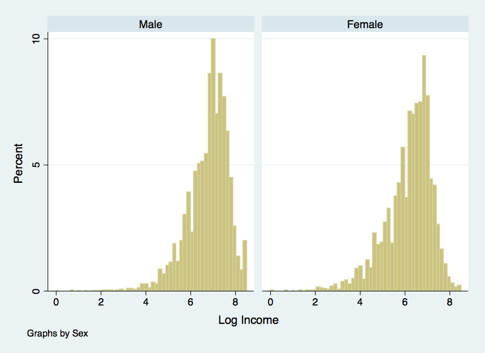
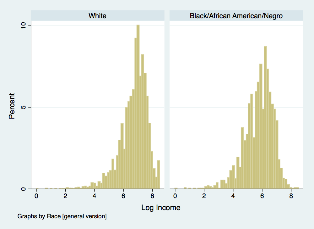
There is something a little deceptive about these income distributions. Recall one of our problems with using log income when estimating mobility rates: individuals reporting zero income are dropped since you cannot take the log of zero. To understand why this is a bit problematic, we will summarize income and log income by race and generate a variable to designate individual’s reporting an income of zero:
. gen zero_income = 0 if income>0 & income~=.
(932,456 missing values generated)

. replace zero_income = 1 if income==0
(595,645 real changes made)

. * Note that race==1 for white and race==2 for black
. sum income ln_income zero_income if age>24 & age<60 & race==1

    Variable │        Obs        Mean    Std. Dev.       Min        Max
─────────────┼─────────────────────────────────────────────────────────
      income │    550,492    569.5389    863.4532          0       5001
   ln_income │    264,937    6.745254     .932867          0   8.517393
 zero_income │    550,492    .5187269    .4996496          0          1

. sum income ln_income zero_income if age>24 & age<60 & race==2

    Variable │        Obs        Mean    Std. Dev.       Min        Max
─────────────┼─────────────────────────────────────────────────────────
      income │     55,962    254.9826    387.8304          0       5001
   ln_income │     29,878    5.783654    .9809142          0   8.517393
 zero_income │     55,962     .466102    .4988541          0          1
Notice that the fraction of white adults with an income of zero is larger than the fraction of black adults with an income of zero. This might seem odd at first, suggesting that employment outcomes were better for black adults than for white adults. However, there are two other things that may be going on here. Let’s dig a little deeper into the data.
. gen zero_income_overall = zero_income
(336,811 missing values generated)

. replace zero_income_overall = 0 if incnonwg == 2
(167,864 real changes made)

. sum income ln_income zero_income zero_income_overall if age>24 & age<60 & race==1

    Variable │        Obs        Mean    Std. Dev.       Min        Max
─────────────┼─────────────────────────────────────────────────────────
      income │    550,492    569.5389    863.4532          0       5001
   ln_income │    264,937    6.745254     .932867          0   8.517393
 zero_income │    550,492    .5187269    .4996496          0          1
zero_incom~l │    550,492    .3621506    .4806225          0          1

. sum income ln_income zero_income zero_income_overall if age>24 & age<60 & race==2

    Variable │        Obs        Mean    Std. Dev.       Min        Max
─────────────┼─────────────────────────────────────────────────────────
      income │     55,962    254.9826    387.8304          0       5001
   ln_income │     29,878    5.783654    .9809142          0   8.517393
 zero_income │     55,962     .466102    .4988541          0          1
zero_incom~l │     55,962     .306458    .4610263          0          1
What we have done above is account for non-wage income in addition to wage and salary income. This has reduced the fraction of both black and white individuals with no income, but has not eliminated the black-white gap. Let’s look at one last thing:
. * Note that sex==1 for male and sex==2 for female
. sum income ln_income zero_income zero_income_overall if age>24 & age<60 & race==1 & sex==1

    Variable │        Obs        Mean    Std. Dev.       Min        Max
─────────────┼─────────────────────────────────────────────────────────
      income │    276,068    950.8008    997.8441          0       5001
   ln_income │    201,118    6.872841    .8839883          0   8.517393
 zero_income │    276,068    .2714911    .4447296          0          1
zero_incom~l │    276,068    .0639516    .2446672          0          1

. sum income ln_income zero_income zero_income_overall if age>24 & age<60 & race==2 & sex==1

    Variable │        Obs        Mean    Std. Dev.       Min        Max
─────────────┼─────────────────────────────────────────────────────────
      income │     26,760    406.3284    456.4466          0       5001
   ln_income │     18,996    6.040882    .8731689          0   8.517393
 zero_income │     26,760    .2901345    .4538328          0          1
zero_incom~l │     26,760     .082997    .2758829          0          1
Now we are looking just at adult males. Notice that our employment gap has reversed, white males are less likely to have zero income than black males, and our income gap has become more pronounced. The different labor force participation patterns of white and black females have substantial impacts on what the summary statistics look like and any inferences based on those statistics.
Now let’s take advantage of the educational attainment data and think about wage gaps by education level. First, let’s see how the educational attainment data is coded:
. tab educ, sum(educ)

Educational │
 attainment │  Summary of Educational attainment
   [general │          [general version]
   version] │        Mean   Std. Dev.       Freq.
────────────┼────────────────────────────────────
  N/A or no │           0           0     183,660
  Nursery s │           1           0     202,223
  Grade 5,  │           2           0     500,947
    Grade 9 │           3           0      77,531
   Grade 10 │           4           0      80,394
   Grade 11 │           5           0      50,453
   Grade 12 │           6           0     161,625
  1 year of │           7           0      20,790
  2 years o │           8           0      24,484
  3 years o │           9           0      10,416
  4 years o │          10           0      28,581
  5+ years  │          11           0      10,628
────────────┼────────────────────────────────────
      Total │   2.8246465   2.4416302   1,351,732
We will start by generating indicator variables for several educational categories: eight years or less, some high school, high school grad, some college, college grad.
. gen common_school = 0 if educ~=.

. replace common_school = 1 if educ<3
(886,830 real changes made)

. gen some_hs = 0 if educ~=.

. replace some_hs = 1 if educ>2 & educ<6
(208,378 real changes made)

. gen hs_grad = 0 if educ~=.

. replace hs_grad = 1 if educ==6
(161,625 real changes made)

. gen some_col = 0 if educ~=.

. replace some_col = 1 if educ>6 & educ<10
(55,690 real changes made)

. gen col_grad = 0 if educ~=.

. replace col_grad = 1 if educ>9
(39,209 real changes made)
Now we can run a really simple regression capturing the relationship between education and log earnings, giving us an estimate of the returns to education:
. reg ln_income common_school some_hs some_col col_grad if age>24 & age<60

      Source │       SS           df       MS      Number of obs   =   295,886
─────────────┼──────────────────────────────────   F(4, 295881)    =   6550.75
       Model │  23214.2056         4   5803.5514   Prob > F        =    0.0000
    Residual │  262131.912   295,881  .885936954   R-squared       =    0.0814
─────────────┼──────────────────────────────────   Adj R-squared   =    0.0813
       Total │  285346.118   295,885  .964381829   Root MSE        =    .94124

──────────────┬────────────────────────────────────────────────────────────────
    ln_income │      Coef.   Std. Err.      t    P>|t|     [95% Conf. Interval]
──────────────┼────────────────────────────────────────────────────────────────
common_school │  -.4758037   .0048874   -97.35   0.000    -.4853829   -.4662245
      some_hs │  -.1698294   .0059714   -28.44   0.000    -.1815331   -.1581257
     some_col │   .1265731   .0080291    15.76   0.000     .1108363    .1423098
     col_grad │   .4394552   .0080426    54.64   0.000     .4236919    .4552186
        _cons │   6.892993   .0042761  1611.97   0.000     6.884612    6.901374
──────────────┴────────────────────────────────────────────────────────────────
Notice that I included all of the indicator variables for education levels except for high school grad. In general, when you are including indicator variables to capture different values for a categorical variable, you must omit one indicator. If you do not, you will run into a big problem of multicollinearity and the coefficients cannot be uniquely identified. In practice, Stata will drop one of the variables in this case so that the regression can be run but it is nicer to choose for yourself which category to omit. The coefficients on the included indicator variables then measure the difference in the outcome relative to to the omitted category. So in this case, the coefficient on col_grad is measuring the additional earning for a college grad relative to a high school grad.
Now let’s do a slightly better job of estimating the returns to education by including controls we know influence earnings. We will construct variables for experience, age squared, and experience squared and generate indicators for race and sex:
. gen experience = age - (higrade + 2)

. replace experience = age - 5 if higrade == 1
(183,660 real changes made)

. gen age_2 = age^2

. gen experience_2 = experience^2

. gen female = 0 if sex==1
(674,165 missing values generated)

. replace female = 1 if sex==2
(674,165 real changes made)

. gen black = 0 if race==1
(143,180 missing values generated)

. replace black = 1 if race==2
(137,114 real changes made)
Now we can run a better version of the above regression:
. reg ln_income common_school some_hs some_col col_grad age age_2 experience experience_2 black female if age>24 & age<60

      Source │       SS           df       MS      Number of obs   =   294,815
─────────────┼──────────────────────────────────   F(10, 294804)   =  10277.19
       Model │  73447.3598        10  7344.73598   Prob > F        =    0.0000
    Residual │  210685.755   294,804  .714663829   R-squared       =    0.2585
─────────────┼──────────────────────────────────   Adj R-squared   =    0.2585
       Total │  284133.115   294,814  .963770768   Root MSE        =    .84538

──────────────┬────────────────────────────────────────────────────────────────
    ln_income │      Coef.   Std. Err.      t    P>|t|     [95% Conf. Interval]
──────────────┼────────────────────────────────────────────────────────────────
common_school │  -.0835449   .0073238   -11.41   0.000    -.0978994   -.0691905
      some_hs │   -.048543   .0059165    -8.20   0.000    -.0601391   -.0369469
     some_col │  -.0521658    .007554    -6.91   0.000    -.0669715   -.0373601
     col_grad │   .0161879   .0088892     1.82   0.069    -.0012348    .0336105
          age │   .1919434   .0030665    62.59   0.000     .1859332    .1979536
        age_2 │  -.0011768   .0000322   -36.57   0.000    -.0012398   -.0011137
   experience │  -.0895515   .0018664   -47.98   0.000    -.0932097   -.0858934
 experience_2 │   .0000886   .0000233     3.80   0.000      .000043    .0001343
        black │  -.5867135   .0055239  -106.21   0.000    -.5975401   -.5758869
       female │   -.629986   .0036412  -173.02   0.000    -.6371227   -.6228493
        _cons │   3.509519    .047373    74.08   0.000     3.416669    3.602368
──────────────┴────────────────────────────────────────────────────────────────
This now gives us a better estimate of the returns to education and gives us estimates of gender and racial gaps in earnings after controlling for education, age and experience levels. However, there is still a pretty big problem. Average incomes and average education levels differ substantially across regions (check this for yourself with the data). This is going to potentially bias many of our coefficients. We should probably be controlling for region. We can do this in the same way we did for our education categories, generating a series of indicator variables and including all of them (except for one) in the regression. However, we can also take a shortcut by using Stata’s interactive expansion command. This command will create indicator variables for any categorical variable:
. xi: reg ln_income common_school some_hs some_col col_grad age age_2 experience experience_2 black female i.region if age>24
> & age<60
i.region          _Iregion_11-42      (naturally coded; _Iregion_11 omitted)

      Source │       SS           df       MS      Number of obs   =   294,815
─────────────┼──────────────────────────────────   F(18, 294796)   =   6596.68
       Model │  81584.2695        18  4532.45942   Prob > F        =    0.0000
    Residual │  202548.846   294,796   .68708139   R-squared       =    0.2871
─────────────┼──────────────────────────────────   Adj R-squared   =    0.2871
       Total │  284133.115   294,814  .963770768   Root MSE        =     .8289

──────────────┬────────────────────────────────────────────────────────────────
    ln_income │      Coef.   Std. Err.      t    P>|t|     [95% Conf. Interval]
──────────────┼────────────────────────────────────────────────────────────────
common_school │  -.1471102   .0072418   -20.31   0.000     -.161304   -.1329163
      some_hs │  -.0786446   .0058154   -13.52   0.000    -.0900426   -.0672466
     some_col │   .0007922   .0074359     0.11   0.915     -.013782    .0153664
     col_grad │   .0793048   .0087917     9.02   0.000     .0620734    .0965362
          age │   .1665501   .0030321    54.93   0.000     .1606072     .172493
        age_2 │  -.0010157   .0000316   -32.10   0.000    -.0010778   -.0009537
   experience │  -.0706882   .0018541   -38.12   0.000    -.0743222   -.0670541
 experience_2 │  -.0000502   .0000229    -2.19   0.029    -.0000951   -5.18e-06
        black │  -.4934027   .0056127   -87.91   0.000    -.5044034    -.482402
       female │  -.6369779   .0035749  -178.18   0.000    -.6439847   -.6299711
  _Iregion_12 │   .0927184   .0063393    14.63   0.000     .0802935    .1051432
  _Iregion_21 │  -.0044005   .0064506    -0.68   0.495    -.0170434    .0082425
  _Iregion_22 │  -.3026446   .0076456   -39.58   0.000    -.3176298   -.2876595
  _Iregion_31 │  -.1532237   .0071458   -21.44   0.000    -.1672292   -.1392181
  _Iregion_32 │  -.4111879   .0084058   -48.92   0.000     -.427663   -.3947127
  _Iregion_33 │  -.3893858   .0078546   -49.57   0.000    -.4047805   -.3739911
  _Iregion_41 │  -.2731964   .0108344   -25.22   0.000    -.2944315   -.2519614
  _Iregion_42 │  -.0740597   .0076829    -9.64   0.000     -.089118   -.0590014
        _cons │   3.988974   .0471479    84.61   0.000     3.896565    4.081382
──────────────┴────────────────────────────────────────────────────────────────
Now we get college education premiums that look a bit more reasonable.